1 Contracts and cost models
When I use a word, it means just what I choose it to mean — neither more nor less.
Lewis Carroll, Through the Looking-Glass (1871)
1.1 Nine balls and a balance scale
Before any data structure, one question decides everything: what does an algorithm actually promise, and at what price? Both halves need sharpening. This chapter starts with the price: first what a price consists of, then how to say how big one is. Then it turns to the promise, and what a promise is worth when nobody has said what it assumes.
Start with a puzzle where the price is small enough to count on one hand.
You have nine balls. One is slightly heavier; the rest are identical. You have a balance scale that tells you which pan is heavier, or that they match. Find the heavy ball. What is the fewest weighings that always works, and how do you know you cannot do better?
Five minutes and a pen. You’re done when you have a number and a reason nobody can beat it. The reason is the harder half, and it is the half this chapter is about.
Most people find the heavy ball among nine in two weighings by splitting into three groups of three. Fewer can say why two is optimal, and that “why” is the primitive.
1.1.1 Every weighing, drawn out
Each weighing has three possible outcomes: left heavier, right heavier, or balanced. A strategy is therefore a ternary decision tree (each question splits three ways). A tree with \(w\) levels of questions, its depth, has at most \(3^w\) leaves, the end points where the answer is known. To tell \(n\) balls apart you need at least \(n\) distinct leaves, so \(3^w \ge n\), which means at least \(\lceil \log_3 n \rceil\) weighings. No cleverness escapes it.
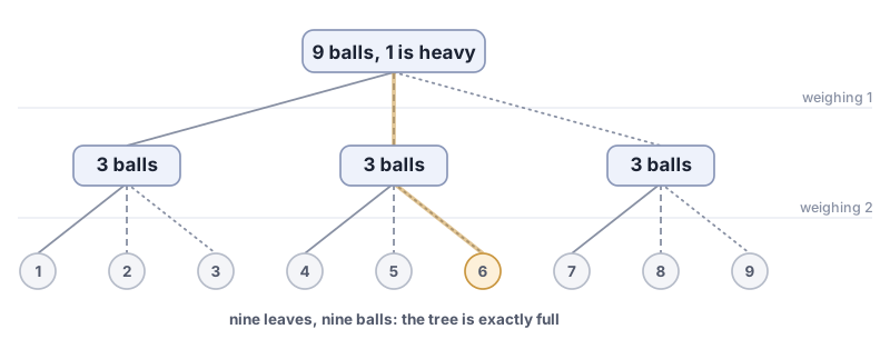
Primitive: the adversary / decision-tree lower bound. When every step yields one of \(b\) answers, \(w\) steps produce at most \(b^w\) distinct outcomes. If the task needs \(N\) distinct outcomes, then \(w \ge \log_b N\), no matter the algorithm. The adversary in the name is an imagined opponent who, at every step, gives the answer that keeps the most outcomes still open.
Ternary division meets that bound exactly: split into three near-equal groups, weigh two, and the odd ball is in the group the scale points to (or the one left off). A solver that does this never needs more than \(\lceil \log_3 n \rceil\) weighings, wherever the odd ball is.1 This is the same primitive as binary search, where each yes-or-no answer gives \(b = 2\) and you need \(\log_2 n\) questions.
1.1.2 Why no sort can be faster
The same count settles something far larger than a puzzle. A comparison sort learns about its input only by comparing two items at a time (“is this one smaller than that one?”), so it too is a decision tree, with \(b = 2\). It has to tell apart all \(n!\) possible orderings of its input, because each one needs a different rearrangement to put it in order, so it needs at least \(\log_2(n!)\) comparisons: a number that, once \(n\) is any size worth caring about, grows very nearly like \(n \log_2 n\). That is a floor under every comparison sort that will ever be written, including the ones nobody has thought of.
Hold onto that sentence. The shorthand for saying it arrives under “How fast does the cost grow?”, and reading that shorthand correctly is the part most people get wrong.
1.1.3 The same trick, everywhere
The decision-tree primitive is a certificate factory (a certificate being proof you can check for yourself): it turns “I cannot see how to do better” into “no one can, here is the proof.” It recurs whenever each answer comes from a short, fixed list of possibilities, and you have already met it three times:
- Ball weighing composes it with divide and conquer: divide into three, and the lower bound says three-way division is optimal.
- Comparison sorting composes it with counting orderings (\(n!\)) to bound every such sort at once.
- Searching a sorted array of \(n\) items needs at least \(\log_2 n\) comparisons, for the same reason: each comparison answers yes or no, and \(n+1\) possible answers have to be told apart, one for each position and one more for “not here at all”.
The move to take with you: count the outcomes the task demands, count the outcomes one step supplies, and divide their logarithms. For the nine balls: nine outcomes needed, three per weighing, and the ratio is two. That single ratio is a lower bound you can state before writing any code.
The idea of a certificate works on answers, not only on bounds. A lower bound is a certificate that nobody can do better; a sorted list beside the input it rearranges is a certificate that this particular answer is right. Either way, what you are handed is something you can check yourself, instead of a claim you have to take on trust.
1.1.4 Three tools we reuse
Three more primitives set the language we will reuse everywhere:
- Loop invariant. A property that is true before a loop starts and stays true after every pass through it; at the end, it proves the answer correct. Binary search keeps “the target, if present, lies in
[lo, hi]”, the stretch of the sorted list between positionsloandhi, true throughout. - Monovariant. A whole number that strictly moves one way and cannot pass a limit proves termination. Each weighing shrinks the candidate set, whose size cannot go below one, so the process must end.
- Splitting the problem. When a method solves a big case by solving smaller copies of itself, its cost is settled by a race: the work done splitting and recombining at the top, against the work piling up in all the small pieces at the bottom. Whichever side is heavier sets the cost. When the two are even, every level costs about the same, and the cost is one level’s work times the number of levels. Binary search is the even case: a little work at each level and one piece left, so its cost grows only with the number of levels, \(\log_2 n\).
1.2 What an algorithm actually spends
1.2.1 Resources
You just counted weighings. Nobody told you to, and nobody had to: on that puzzle the scale is the only thing that is scarce, so weighings are the only thing worth counting. Give that idea its name. A resource is whatever a computation consumes that can run out, and the one that matters is whichever runs out first.
Which one that is depends on the machine and the job, not only on the algorithm. The same code can be limited by a different resource on a laptop, on a phone, and on a rack of machines in a data center. The ones that come up in this book, roughly in the order you will meet them:
- Time: steps taken, however a step is defined. The default, and the one people mean when they say “faster.” Every chapter counts it.
- Space: how much has to be held at once. Sometimes space alone is the limit: a summary that fits in memory beats an exact answer that does not, which is the entire argument for the small summary structures (sketches) later in the book.
- Block transfers: trips to somewhere slow. Disks and networks hand over a whole block at a time, so the count that matters is not how many bytes you looked at but how many trips you made. A structure can do more arithmetic and still win by making fewer trips. This is what the B-tree, in the next chapter, is for.
- Comparisons, probes, queries: steps of a specific kind, counted when that kind is the expensive one. Weighings, in the puzzle above. Comparisons, in the sorting bound. Probes into an array, in binary search. Counting one specific operation is what lets you prove a lower bound at all, because it pins down what an algorithm is allowed to learn per step.
- Random bits: coin flips. Some structures buy their guarantee with randomness instead of bookkeeping, and then randomness is a thing being spent.
- Messages and bandwidth: messages sent, and bandwidth, how much data can cross per second. When the computation is spread across machines, what crosses between them usually dominates everything happening inside them.
- Work and span: when many processors run at once, one number stops being enough: total work done, and the longest chain of steps that must happen in order. The frontier map at the end of this chapter says more.
1.2.2 Trade-offs and cost models
Two things follow from that list, and they are the reason to count resources at all.
The resources trade against each other. Spending space to save time is the oldest move in the book: an index is exactly that. Spending time to save space is the next oldest; so is spending accuracy to save both. Call each thing a design is measured by an axis: time is one, space another, accuracy a third. There is rarely a design that wins on every axis, and a chapter that seems to find one is usually hiding the axis it lost on.
Every cost is a cost in a model, and the model is an assumption. Calling something a fixed-price operation, one that costs the same no matter how much data you are holding, is never free of assumptions: the claim counts some operations and ignores others. The model most cost claims use is the RAM model, in which every memory read is one step. In a real machine a memory read is something else entirely. When a cost claim surprises you, the model is the first place to look, and the model that surprises people most is the one about memory, which comes next.
1.2.3 The memory hierarchy
The RAM model says reading a value from memory costs one step, the same one step, wherever the value happens to be. No real machine has ever worked that way, none does now, and none ever will. This is the part worth understanding rather than memorizing. Engineers have not simply forgotten to fix it. Two forces that cannot be bargained with, physics and economics, both push in the same direction. What they push into existence is a memory hierarchy: a short ladder of places data can sit. Each level is slower than the one above it, and bigger and cheaper per byte, usually by something like an order of magnitude (about ten times), and at one step, the drop from memory to flash, by a great deal more [1]. Where that jump falls turns out to matter more than any of the individual numbers, which is why the table below is worth reading for its gaps rather than its digits.
Take one clock cycle of a processor core as the unit. A cycle is the processor’s basic beat, the time one simple step takes; on a machine running at a few gigahertz (a few billion cycles a second) it is a small fraction of a nanosecond. Everything else is a multiple of that.
The last column is the one that builds the feeling. Stretch a cycle out until it takes one second, and scale everything else by the same factor, so the ratios stay as they are and the numbers land in units a person has lived through. The top rows are memories on the processor chip itself: registers, which hold the values being worked on right now, and the caches L1 to L3, small fast memories that keep copies of recently used data.
| where the data is | how long it takes | vs. one cycle | if a cycle were one second |
|---|---|---|---|
| register, L1 cache | about a cycle | \(\times 1\) | a second |
| L2 cache | a few nanoseconds | \(\times 10\) | ten seconds or so |
| L3 cache | tens of nanoseconds | \(\times 10^2\) | about a minute |
| main memory (DRAM) | around a hundred nanoseconds | \(\times 10^{2\text{–}3}\) | a few minutes |
| flash (SSD) | tens of microseconds | \(\times 10^5\) | a day or two |
| another machine in the same building | hundreds of microseconds | \(\times 10^{5\text{–}6}\) | days to weeks |
| a seek on a spinning disk | milliseconds | \(\times 10^7\) | months |
| a machine on the other side of the planet | around a hundred milliseconds | \(\times 10^{8\text{–}9}\) | a decade |
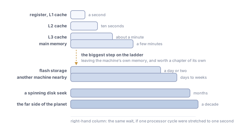
Read the last column once and the point of the section is made. A program that goes to main memory for every value is a person who stops work for a few minutes on every single line. A program that goes to disk for every value has stopped for months. Differences this large are too big to wave away as “only a constant factor”, a phrase that returns, made precise, in “How fast does the cost grow”.
The digits in that table will go stale, and the shape will not. Absolute latencies (how long one access takes) move, levels get inserted (flash was not always there; memory attached over a fast link that keeps all the caches’ copies in agreement is being inserted now), and levels fall out of use (spinning disks have left many systems entirely). What does not move is the ordering, the order-of-magnitude gaps between neighbors, and the fact that any level invented tomorrow will slot into the same hierarchy and obey the same rule. That is why this book prints ratios and units named in words (“a few minutes”, “months”) instead of numbers with decimal points.
1.2.4 ★ Why the hierarchy is unavoidable advanced
Three separate constraints, all pushing the same way.
Distance is time. In one cycle of a few-gigahertz clock, light travels something like ten centimetres in vacuum, and a signal in metal travels less. Anything physically farther away than that cannot possibly answer within a cycle, no matter who builds it or what it is made of. That is the hard floor under the whole table, and it is the reason the bottom rows are what they are: a machine on the other side of the planet is slow because the planet is that size.
On a chip, wires are the problem, not transistors. Shrinking a transistor makes it faster. Shrinking a wire does not. A thinner wire has more electrical resistance, so a signal crawls along it. Transistors have got faster decade after decade; the delay of a long wire across a chip has stubbornly refused to improve the way transistors have. So the cost of reaching across a chip keeps mattering more, not less.
Fast, dense, cool: pick fewer than three. (Dense means many bits packed into a small area.) A fast memory cell is a big one: static RAM spends roughly six transistors per bit and holds its value actively. A dense cell is a slow one: dynamic RAM spends about one transistor and a capacitor per bit and has to be refreshed. Flash is denser again and slower again. And fast circuits switch more often, switching costs energy, energy leaves as heat, and heat leaves through a surface, so the fast region has to stay physically small or it cooks.
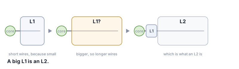
Now put those together, because the conclusion is the one that matters. Suppose you want a large, fast memory. Making the fast tier bigger makes it physically larger, which makes its wires longer, which makes it slower: at which point it is no longer the fast tier. You cannot have a big L1 cache. A big L1 cache is an L2. Levels exist because a single large fast memory is not a thing that can be built, not a thing nobody has bothered to build.
Even suppose the physics relented. The money would not.
Cost per byte falls roughly as fast, level by level, as latency rises. Both follow from the same three constraints, seen from the accounting side: cheap-per-byte is what dense, slow and cool buys you. So a machine built entirely from the top level would cost an absurd amount for a tiny capacity, and a machine built entirely from a bottom level would be affordable, enormous and unusable.
Which means any builder trying to get the most useful machine for a fixed budget lands on the same answer: a little of the fast stuff, more of the middling stuff, a great deal of the cheap stuff, and some scheme for keeping the data you are about to want near the top. Nobody chose this shape. It is what falls out when you minimize cost under those constraints, and it will fall out the same way for hardware nobody has designed yet.
1.2.5 ★ Accelerators advanced
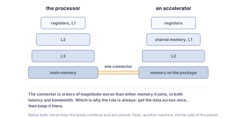
A GPU (a graphics processor, now used for much more than graphics) is not an exception to any of this, and the way it is not an exception is instructive. It has its own levels, in the same order and with the gaps just as wide: a very large register file, then shared memory for each group of threads, and L1, then L2, then the high-bandwidth memory sitting on the package, then across a bridge to the host’s memory, and from there down the host’s entire hierarchy as before.
Two things about that are worth carrying.
The bridge decides the program. The hop between the accelerator’s own memory and the host’s crosses a physical connector, and it is orders of magnitude worse than anything on the device in both latency and bandwidth. Which is why almost every rule of thumb in accelerator programming is some version of get the data across once and keep it there: an algorithm with a worse operation count that crosses the bridge fewer times routinely wins by a margin that no amount of better arithmetic can recover.
A GPU answers the same physics differently, not better. It does not try to make one memory access fast. It runs enormous numbers of threads and switches between them, so that while some are waiting for memory others are working: the latency is still there, in full, and is being hidden behind bandwidth rather than removed. That trade is why GPUs want work shaped as many independent pieces touching memory in regular, adjacent patterns, and why an algorithm full of unpredictable jumps runs badly on one even when its operation count is excellent.
Everything above generalizes to the rest of the zoo. A machine with a CPU, one or more accelerators, a neural processing unit and memory attached over an interconnect is several hierarchies, joined at their slow ends. Adding devices adds levels; it has never yet removed one, and the two forces above say it will not. The safe prediction about hardware that does not exist yet is this: it will have a hierarchy, for the same reasons, in the same shape.
1.2.6 Consequences for algorithms
Two programs with identical operation counts can differ by orders of magnitude, and usually the difference is that one of them walks through memory in order while the other jumps around. The count was never the whole cost; where the data was, and how often it had to move, was the rest of it.
That is why a single cost model is not enough, and why this book uses more than one. Counting steps is the default. Counting block transfers (trips to a slower level, each bringing back a whole block whether you wanted all of it or not) is the model that explains why a structure doing more arithmetic can be faster, and it is the model a later chapter switches to when it builds the B-tree. Counting transfers without knowing the block size is a third model, which the frontier map at the end of this chapter points at. A structure that turns scattered writes into sequential ones, like the LSM-tree in the search chapter, is answering the same pressure from another side.
The habit to build: before asking how many operations something does, ask where the data lives, and how many times it has to move. On modern hardware that question is usually the one that decides the answer.
1.3 How fast does the cost grow?
Back to counting, now that there is something honest to count. Once you have picked the resource (steps, bytes held, trips to a slower level) one question is left, and it is the one every cost claim in this book is an answer to: how does that count grow as the input gets bigger? Nobody cares about the count at \(n = 10\). Everybody cares what happens at \(n = 10\) million.
1.3.1 At most, at least, exactly
Three symbols carry this, and they say three different things about a count \(f(n)\):
- \(O(g(n))\): no worse than \(g\), for large \(n\), ignoring constant factors. An upper bound, and a promise: it will not cost more than this.
- \(\Omega(g(n))\): no better than \(g\). A lower bound, and usually a piece of bad news: the count never drops below this.
- \(\Theta(g(n))\): both at once. The growth is pinned: no worse and no better. When you know this much, say this, not \(O\).
“Ignoring constant factors” is doing real work in all three. \(\Theta(n)\) says nothing about whether a step takes a nanosecond or a minute; it says that doubling \(n\) roughly doubles the total, once \(n\) is large. Constants decide which of two programs you ship. Growth decides which of them still works next year.
1.3.2 What each growth rate feels like
The table below is about a count, whatever is being counted: weighings, comparisons, bytes held, trips to disk. That is why the resources came first: you pick the resource, then you use this table once, for any of them.
The budget column assumes a machine doing a billion steps a second and one second of patience. It is a rough number and it is meant to be: the point is the shape, not the digits.
| growth | when \(n\) doubles, the cost | \(n\) affordable in a second | the feeling |
|---|---|---|---|
| \(1\) | does not move | anything at all | free; size never enters it |
| \(\log n\) | goes up by one step | anything you can store | practically free, forever |
| \(\sqrt{n}\) | grows by about 40% | \(10^{18}\) | comfortable, quietly growing |
| \(n\) | doubles | \(10^9\) | fair: you looked at everything once |
| \(n \log n\) | a shade more than doubles | \(4 \times 10^7\) | the working limit of “still fine” |
| \(n^2\) | quadruples | \(30{,}000\) | fine in testing, dead in production |
| \(n^3\) | goes up eight times | \(1{,}000\) | only ever for small \(n\), and you know it |
| \(2^n\) | squares | \(30\) | one more item doubles everything |
| \(n!\) | worse than squares | \(12\) | a wall, not a slope |
Those are shapes. Here is each one as something you have felt:
- \(\mathbf{1}\): reaching for a light switch you have used a thousand times. The size of the room never came into it.
- \(\log n\): guessing a number between one and a million by halving the range. A million possibilities, twenty guesses. Widen it to two million and you ask one more question.
- \(\sqrt{n}\): a filing cabinet with \(\sqrt{n}\) drawers holding \(\sqrt{n}\) files each: scan the drawer labels, then scan one drawer. Twice the files makes each of those jobs 40% longer, not twice as long.
- \(n\): reading every name on the guest list to find one person. Twice the guests, twice the reading. Nothing clever, nothing pathological.
- \(n \log n\): sorting a deck by merging piles. Every card is handled, and handled once per doubling of the pile it is in. Barely worse than reading them all, which is why this is the workhorse of the whole field.
- \(n^2\): every guest shakes hands with every other guest. The tenth guest adds nine handshakes; the hundredth adds ninety-nine. Each new arrival costs more than the last one did, and that is the part that kills you: it is fine at the size you tested and hopeless at the size you shipped.
- \(n^3\): the same handshakes, but every handshake has to be witnessed by every guest.
- \(2^n\): deciding, for each guest separately, invite or don’t, and examining every possible guest list. One more name on the list doubles the work. Not once. Every single time.
- \(n!\): seating every guest in every possible order. Twelve guests is about half a second. The thirteenth guest makes it six seconds, the fourteenth a minute and a half. Twenty guests is a human lifetime. Twenty-six is the age of the universe.
The gap between the last two rows and everything above them is not a difference of degree. Every row down to \(n^3\) is a program that gets slower as the data grows. \(2^n\) and \(n!\) are programs that stop working, and a machine ten times faster moves the wall by three items for \(2^n\), and by one for \(n!\).
1.3.3 Worst, average, amortized, expected, w.h.p.
The symbol says how a count grows. It does not say which run you are counting. That is a separate question, and five phrases answer it all through this book. Any of them can be attached to any of the growth rates above:
- Worst case. The most expensive input of that size. The default in this book, and the only one that holds for every input on every run.
- Average case. Averaged over inputs, under some stated distribution of them: an assumption about how likely each input is. Only as good as that stated distribution, which is usually the assumption that breaks.
- Amortized. Averaged over a run of operations on one structure, not over inputs. It says a long sequence is cheap in total, and says nothing about the one operation you are waiting on. A growable array is the classic case, and “Push on it” has you prove it.
- Expected. Averaged over the algorithm’s own coin flips, for a fixed input. Different from average case in the way that matters: nobody chooses the input to make it bad, because the randomness is yours, not the adversary’s.
- With high probability (w.h.p.). Not an average at all: the bound holds except on a vanishingly small fraction of coin flips. Stronger than expected, and the thing randomized structures actually promise.
“\(O(1)\) amortized” and “\(O(1)\) worst case” are different promises about the same growth rate, and systems have been taken down by reading one as the other.
1.3.4 Slow code or a hard problem?
One more distinction, because it is the single most common misreading in the subject. A bound can be about one algorithm, or about a whole problem.
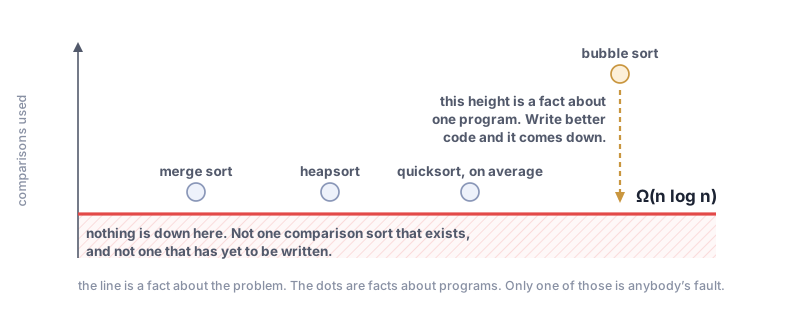
“This algorithm takes \(\Omega(n^2)\) steps” says this code is slow. Write better code.
“Sorting by comparisons takes \(\Omega(n \log n)\) comparisons” says no code can do better, ever, including code nobody has written. That is what the decision-tree count in “Why no sort can be faster” actually proved, and it is why that proof was worth doing: it is a statement about the problem, not about anybody’s attempt at it.
Someone tells you they have a sorting algorithm that runs in \(O(n \log n)\), and someone else tells you bubble sort runs in \(O(n \log n)\). One of those is ordinary; the other is wrong. Before reading on, say which, and say exactly which of the two kinds of bound above is being confused with which.
Bubble sort is not \(O(n \log n)\). The \(\Omega(n \log n)\) result is a lower bound on the whole class of comparison sorts, not an upper bound on any one algorithm in it. A floor under everybody says nothing about how high above the floor one particular algorithm sits. Bubble sort makes about \(n^2/2\) comparisons; it is quadratic, and the lower bound is perfectly happy about that.
Confusing a class lower bound with one algorithm’s cost is the one error never to make.
1.4 When there is no single best
Everything so far has been about measuring: which resource, how the count grows, whether a bound is about a program or a problem. Measuring is the easy half. The hard half starts the moment two measurements disagree.
Here is the disagreement, in its smallest form. One design answers every query exactly and needs a gigabyte of memory to do it. Another answers approximately and is wrong in one direction only (it may say “yes” when the true answer is “no”, never the reverse), and fits in a few megabytes. Which is better?
The question has no answer. Not “no answer yet”: no answer of that kind. Ask it about a bank’s ledger and the exact one wins without discussion. Ask it about a router deciding in nanoseconds whether a packet is worth a closer look, and the small one wins just as easily. Nothing about either design changed in between.
School trains you to expect a single best answer. Every optimization problem you were given had one number to minimize. Real numbers are totally ordered: given any two, one is bigger, so among any finite set of candidates “the best” exists. Design has no such number. It has several, they move against each other, and there is no natural exchange rate between a megabyte and a microsecond.
1.4.1 Domination and the Pareto frontier
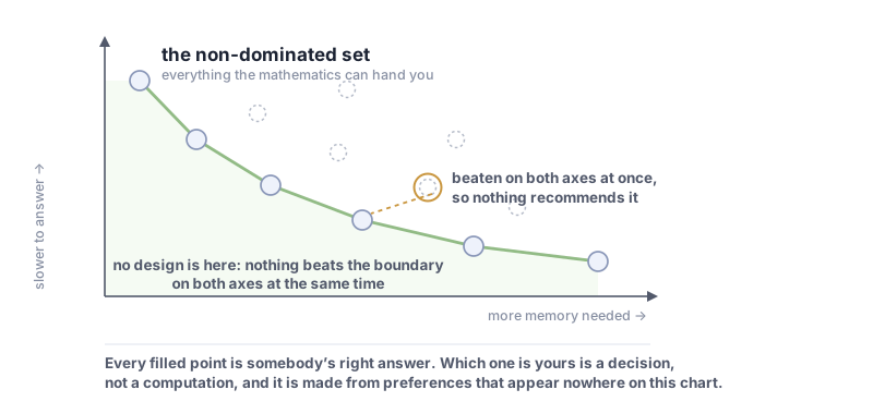
Only one way of comparing designs survives. Design A dominates design B when A is no worse than B on every axis and strictly better on at least one. That is the whole of what the mathematics will grant you, and it is genuinely useful: if A dominates B, then B is out, for everybody, in every context, with no discussion of preferences at all. Nobody has a reason to pick a design that something else beats outright.
Apply that everywhere and you are left with the designs nothing dominates. That set is called the non-dominated set, or the Pareto frontier, and it is the real output of an honest analysis. (Nothing to do with the frontier maps that close each chapter of this book: an unfortunate collision of a good word.)
1.4.2 Who chooses, and what got left out
Now the part that matters, and the reason all this sits in a chapter about contracts.
A machine can compute that set. What it cannot do is choose within it for us. Computing the frontier is mechanical work, and it is the sort of work to hand to something faster than you. Picking a point off it is not hard either: a coin does that. But every point on it is unbeaten, so nothing about the picking is a calculation someone failed to perform. It is a statement of preference, and preferences are not in the data. They come from outside: who pays when this is slow, who pays when it is wrong, how often the bad case actually arrives, whether an answer that is late is merely annoying or completely worthless.
Those are answerable questions. They are just not questions about algorithms. No structure is simply best, which is why the useful skill is being able to say which axis you are buying and what you are paying for it, in terms precise enough that somebody can disagree with you.
And one honest edge, because it is where this goes wrong in practice. The axes were a choice too. Draw the picture with memory and time and you will find the frontier for memory and time. Some axes never get drawn. What does it cost to run? How much else breaks when it fails? How long does a new engineer need before they dare touch it? Leave those out and your optimum is perfectly real on the axes you kept, and wrong on the one you dropped. A design that is unbeatable on a chart missing an axis is the most common way good analysis produces a bad system.
That missing axis is precisely what the assumption of a contract is for: the part that says when its promise holds. Contracts are the next thing this chapter builds.
1.5 What a data structure promises
1.5.1 What a data structure is
The chapter has been coming close to one idea without stating it. Both parts of it are already here.
Counting outcomes told you what a single step can tell you: one weighing splits the possibilities three ways, one comparison splits them two ways, and no cleverness gets more out of a step than the step contains. That is a ceiling, and it holds no matter how the data is lying around.
But whether a step actually tells you that much depends entirely on how the data is arranged. One comparison against an unsorted pile of a million keys rules out exactly one key. The same comparison, against the same million keys kept in sorted order, rules out half a million. Identical operation, identical cost, and one of them learns five hundred thousand times as much, because the arrangement made a conclusion available that was not available before. You did not look at the other half a million keys. You did not have to: their order was already known, so the comparison settled them too.
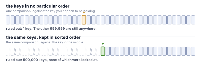
That is what a data structure is. It is an arrangement of data that makes particular conclusions available cheaply, so that algorithms built on top of it can reach further per step than they otherwise could. Not storage, not a container: a standing set of facts that are true about the data, which every operation is then allowed to reason from.
And the sharp edge of that, the part worth carrying into every chapter after this one: a structure makes particular conclusions cheap, and refuses the rest. A sorted array hands you “which half is it in” for free and charges you dearly for “make room for one more.” A hash table (a structure that files each key under a number computed from the key) gives away “is this exact key present” and can answer “what is the next key after this one” only by looking at every key it holds. Answering that question cheaply is exactly what sorted order buys, and a hash table keeps no order. You do not choose a structure by what it holds. You choose it by which inferences you need to be cheap, and which you can afford to give up.
1.5.2 Structures as invariants
The part above said what a structure is for. This one says how you come to have one, and the two halves close into a single idea. Those cheap conclusions are available only because certain things stay true about the data permanently, after every operation anyone ever performs. Sorted order buys you half a million keys per comparison exactly as long as it is still sorted.
You have met this kind of fact once already. The loop invariant from “Three tools we reuse” is a promise one loop keeps on every pass. Here the promise belongs to the data itself, and it has to survive every operation, for as long as the data exists. Taking that idea from a single loop to a whole structure is what this book is organized around.
A data structure is not its code. It is the set of properties it promises to keep, and the conclusions it makes cheap are the ones those properties license.
The argument is easiest to see on a structure that looks, at first, like nothing but arbitrary rules. A red-black tree keeps keys in a branching arrangement and paints each link between two keys either red or black, following rules that stop any branch growing much longer than the others. You will build one later in the book, and nothing here depends on knowing how it works. For now ignore the machinery and read only what it promises. The version this book builds, the left-leaning red-black tree, is exactly five things held true at once:
the keys are in order, the topmost node counts as black, red links always lean left, no two red links ever touch, and every path down crosses the same number of black links.
You do not need to know why those five keep a tree short. You only need to see that they, and not the code, are the structure. Everything else (the color bit, the rotations, the flips) is an encoding, chosen because it makes those five properties cheap to keep. A different encoding keeping the same five properties would be the same structure wearing different clothes.
The payoff shows up immediately. The other famous variant, the one most textbooks teach, is the same list with two items loosened: drop “red links always lean left”, and weaken “no two red links ever touch” so that it forbids only a red link hanging directly below another, not one on each side of the same node. Do both and you have the standard red-black tree (the search chapter’s appendix sets the two side by side). Two structures that look entirely different on the page, with different code and different case analyses, differ by exactly two promises. You cannot see that by comparing implementations. You can only see it by comparing promises.
1.5.3 Specifications: rules and meaning
Once a structure is defined this way, every operation on it stops being code and becomes an obligation:
if the structure was valid (all five rules held) before, it is valid after, and the set of keys changed in exactly this stated way.
That is the whole specification of insert. Any implementation satisfying it is a correct insert, in any language, written by anyone or anything. The implementation comes after the specification, and can be replaced.
You need both halves. Drop the second and an insert that quietly does nothing passes: the structure was valid, and it still is.
The second half, “the set of keys changed in exactly this stated way”, has to be stated in terms of something, and the five rules cannot supply it. Before any rule there is what the tree is for: it holds a set of keys. That set is the structure’s meaning, and each operation is a plain sentence about it. insert(k) leaves the set with k added and nothing else changed; delete(k) leaves it with k gone and nothing else changed. The rules say which trees are allowed. The meaning says which answer comes out. A specification that states only the rules can be met by a program that keeps every rule and gives the wrong answer.
The smallest case of that fits on one line. Specify sorting as “the output is in order.” Before reading on, find a useless program that meets it. Now a sort that ignores its input and returns an empty list meets the specification, because an empty list is in order. So does one that returns a hundred zeros. Add the clause about meaning, “and the output is a rearrangement of the input,” and both are ruled out, because neither holds the items it was given. Nothing was wrong with the first clause. It was true, and it was easy to check. It just said nothing about which answer comes out, and a specification that says nothing about the answer allows any answer that merely looks right.
1.5.4 Where invariants come from
Where do the rules come from, then? Usually from a goal loosened until it can be kept. Binary search wants “the target is at mid,” which it cannot know until the end, so it keeps a weaker promise instead, one it can restore after every probe: “the target, if present, lies in [lo, hi].” That promise is true before the first probe, survives every probe, and at the end, when the range has shrunk to one slot or to nothing, it is the answer. Structures are designed the same way. “Every path down has the same length” cannot survive a single insertion. “Every path down crosses the same number of black links” can, given a repair near the change. So the promises mark out a region: the set of arrangements the structure is allowed to be in. Choosing the region is most of the design. It must be tight enough that every arrangement inside it has the cost you want, and loose enough that an update which steps outside can step back in with a small local repair. The search chapter lays four such regions side by side, in its section on what “balanced” is allowed to mean.
Why design this way. Because it moves the moment of failure earlier. Writing code and then testing it tells you about the cases you thought of. Writing the invariant first tells you something better: the places where you cannot state cleanly what you want are the places your design is confused. A property you can’t write down is a design you haven’t finished. That signal arrives before any code exists, which is the cheapest possible time to get it.
1.5.5 Contracts
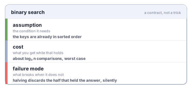
This is also why every reusable idea in this book carries the same three fields:
| field | what it is |
|---|---|
| assumption | the condition under which it holds, the hypothesis |
| cost | the resource bound you get when it does hold |
| failure mode | what breaks when the assumption doesn’t, the thing the promise does not cover |
Those are the three parts of a contract. Without them you have a trick you have memorized; with them you have something you can build on, because you know what it needs and what it refuses to promise.
The contract card (the table above, drawn as a card in the figure below) records a design once it is made. Making a design runs through the same fields as questions, usually in this order:
- What is the workload (the mix of operations the design will face), and what does it ask for most often?
- Which resource is scarce, and so what are you paying for?
- What can no design beat? That is the floor from the decision tree.
- Which promise will you keep, stated on the meaning and not only on the rules?
- Which idea keeps that promise cheap?
- What does it cost, and what does it refuse to cover?
- What change in the workload would make you reconsider?
Every structure in the search chapter answers these seven, and watching it do so is most of what that chapter teaches.
1.6 Checking an answer you did not produce
1.6.1 Checking vs finding
A specification is worth only as much as the checks that can be run against it, and checking turns out to be a different job from finding: usually a much cheaper one.
Take sorting again. Producing a sorted list costs about \(n \log_2 n\) comparisons at the very least; the decision-tree count proved that. Checking a list someone hands you costs one pass: is every item no larger than the next? Whether it holds the same items as the input is one more pass, keeping a tally for each item: add one for each copy in the input, take one away for each copy in the output, and check that every tally ends at zero. That cost grows like \(n\), against \(n \log n\) for the sort, so the check can afford to run every time, even when the sorter is somebody else’s and you cannot read its code.
1.6.2 Reference algorithms and certificates
That gives two kinds of check, and neither depends on how the answer was produced.
- The obvious algorithm as the definition. Some problems have a method so plain that its correctness is not in question: look at every item. It may be far too slow to use, and that does not matter, because its job is to define the right answer on inputs small enough to afford it. The clever method has to agree with it. The book’s companion library (described at the end of this chapter) holds its fast text-search structures to a naive scan of the text in exactly this way, and keeps the scan deliberately naive: a reference that shared the clever idea could share its bug too.
- An answer that carries its own evidence. Some answers can arrive with something cheap to check: the sorted list beside the input, a route beside its length, later in the book a flow beside a cut proving nothing larger exists. Algorithms built to return such evidence are called certifying [2]. You trust the answer because you checked it, not because you trust the program that produced it.
Why insist that the check come from somewhere else? Because two programs written from the same misunderstanding agree with each other. Let the author of a sort also write the test, and a test written from the same misreading of the task passes the same wrong outputs. The check needs a different origin: an obvious algorithm, a version somebody else wrote and checked, a certificate. That is the question to ask of any check, including this book’s own, which is where this chapter ends up.
1.7 ◆ Components and primitives big picture
There are two sizes of thing to carry out of a book like this, and it is worth knowing which one you are being handed.
A finished data structure is a component. You reach for a B-tree, a queue, a cache when you are building a system, the same way you reach for a library. Much of this book teaches exactly that, and it is a real skill.
But you cannot design a new structure out of components. Each one is already the answer to one particular question, with the trade already made and baked in. The moment your question is slightly different, a finished component has nothing to offer you but “close enough.”
The material you can actually build with sits one level down: the small ideas each structure is assembled from. Those are small enough to pull apart and recombine, and (this is the point) they turn up in places with no visible connection to where you first met them. The same idea that keeps a tree short also makes a growable array cheap. The same one that rescues a search tree from a bad input order is the whole of hashing.
This book calls them primitives. They are collected in the catalog, and each chapter ends by taking its structures back apart into them. Six structures is something to remember; ten primitives is something to think with. They are also the words a specification is written in: a contract that says “sorted”, “balanced” or “amortized” is only as precise as those words are.
1.8 ◆ How this book checks itself big picture
Writing an invariant down doesn’t make it true. So: every time the book is built from its source files, each runnable block of code in a chapter that prints its code is copied off the page and run against a companion library, and the build fails if the two disagree. Today that is the search chapter; the others join as they are converted to print their code.
That check exists because of a bug. An early version of a color-flipping routine in the search chapter was printed in this book and was wrong. When a check was finally run on it, the printed routine corrupted 276 of 400 randomly built trees. The companion library, algodesign, had the correct version all along, passing ninety-one tests. The library was never the problem. The page was. Nothing but running the printed code would have caught it.
The Python in that library is the code this book prints: mutable, and the shortest form that stays honest. The Rust beside it is the version written for performance. The Lean beside it is the version written to be proved, as inductive trees and the invariants on them. The page is checked against the Python, because a listing and the file can drift apart, which is what happened to the color flip above. Where a listing is a shorter form of the library function, the check holds them to the same behavior on shared inputs.
The library carries its structures in three languages: Python, Rust, and Lean, a language in which programs, and proofs about them, are checked by machine. The Lean proofs are proofs about the Lean definitions. They are not a proof about the Python and not a proof about the Rust. For selected searching implementations, automated tests compare Lean and Rust invariant checkers and operations, compare Rust and Python results, and check runnable listings from the book against the Python library. These comparisons test agreement on the inputs exercised; they are not proofs that the languages agree on every input. Other parts of the library are checked differently, and wherever the text claims something has been checked, it says how.
Where a claim in the text is backed by a proof, the text says so, and says what the proof does and doesn’t cover: usually less than you’d hope. A proof assistant checks the properties someone thought to state, with complete rigor, and is perfectly silent about the ones nobody stated. Deciding what to state is not a thing a machine does for you.
One rule holds all of this together: what is being checked has no say over the check. The printed code cannot edit the harness it is run against, and the library cannot edit the page it is held to.
Three languages agreeing is weaker evidence than it sounds, because all three were written by one process from one reading of the text. Agreement among them catches a slip in one of them. It cannot catch a misreading they share, and that has happened here. The library’s copy-the-key deletion (see the search chapter’s binary-search-tree deletion section), in all three languages, copied keys down a chain. Having moved the successor’s key up (the successor is the next larger key), it deleted the successor by copying again, where the textbooks cut the successor’s node out of the tree in one step. The three agreed with one another, every proof about the Lean held, and every comparison between them passed. What caught it was a comparison with the textbooks. That is why each structure in the library is tied to a named textbook version: a reference with a different origin.
And a check that cannot fail is not a check, so the one that runs this book’s listings is itself tested first, on deliberately broken copies of the printed code. Some listings are not run at all; “How to use this book” says which.
1.9 ✎ Push on it practice
- Harder puzzle: now the odd ball may be heavier or lighter, and you do not know which. Why does distinguishing \(2n\) possibilities change the bound, and how many weighings does twelve balls need?
- Prove the \(\Omega(n \log n)\) sorting bound cleanly from \(\log_2(n!)\) using Stirling’s approximation.
- For each claim, name the cost model that makes it true or false: “hashing is \(O(1)\)”, “appending to a dynamic array is \(O(1)\)”, “a binary search on disk is fast”.
- Amortization preview: a dynamic array doubles when full. Show that \(n\) appends cost \(O(n)\) total, so \(O(1)\) each on average, even though one append occasionally costs \(O(n)\).
- Three specifications for “remove the smallest item from a collection”: (a) the collection afterwards is one item shorter; (b) the returned item is no larger than anything left; (c) the returned item is no larger than anything left, and the collection afterwards holds exactly the items it held before, minus that one. For each of (a) and (b), write a wrong
remove_minthat satisfies it. Then say why (c) admits no wrong one. Check yourself: aremove_minthat deletes the largest item passes (a); one that returns the smallest item and removes nothing passes (b). - Take the sorting specification from “Specifications: rules and meaning” and drop “is in order” instead of “is a rearrangement of the input”. Name, in one line, a wrong sort the weakened specification now admits.
- Write the checker for a sort’s output: in order, and a rearrangement of the input. Time it against Python’s
sortedon a million random integers, and say how its running time grows with \(n\).
A colleague reports a new algorithm that sorts arbitrary numbers using only pairwise comparisons in \(O(n)\) time. Without running it, argue whether this is possible. If it is not, state exactly which lower bound it violates and why. If it could be, state which assumption of that lower bound it must be breaking.
1.10 ★ Frontier map advanced
- Cache-oblivious algorithms. The RAM model charges \(O(1)\) per memory access, but real memory is a hierarchy. Cache-oblivious algorithms are tuned for block transfers without knowing the block size. Signature: performance that does not match the operation count. Reach for it when constants and locality (whether the data touched next sits near the data touched last) dominate.
- Parallel and work-span models. When many processors run at once, one number is not enough. The work-span model reports total work and the longest dependent chain (the span). Signature: code whose speed depends on how much can happen at the same time. Reach for it when scaling across cores or GPUs.
- Certifying algorithms. Algorithms that return, beside each answer, evidence that the answer is right, which a small and separately trusted checker verifies [2]. Signature: you trust the answer, not the program. Reach for it when the program comes from somewhere you cannot inspect.
- Checks under optimization. When something searches against your check, it finds the check’s gaps, as the preface’s coding agents did. Signature: a score that rises while the thing it measures does not. Reach for it whenever a loop optimizes against a test. Mutation analysis [3] is the standard way to test the tests. This entry belongs to the part of the subject that moves with the technology, and it will date faster than the rest of the chapter.
The book’s solver is
algodesign.contracts.ball_weighing; its test checks every placement of the odd ball.↩︎